1. Could the results be replicated using a genuinely open-source harness?
2. Did the pipeline depend on Sword’s proprietary clinical model, or could a general-purpose LLM stand in for it?
3. Could a newer judge such as GLM-5.2 or DeepSeek improve on the paper’s choice of GLM-4.6?
4. How much would the full experiment cost in API fees and compute?

TL;DR: I reproduced the MindGuard method and am releasing the open-source harness I used to do it. You do not need Sword’s proprietary clinical model. GLM-5.2 slightly outperformed GLM-4.6 in this reproduction, while DeepSeek was nearly identical and far cheaper. The entire study cost about $50.

Question 1: Does it replicate?

Yes. I was able to replicate the method with a newly written harness and a freshly generated training dataset. I am releasing that harness today as the Mental Health Guard Harness.

MindGuard is a distillation pipeline. A large high cost judge model reads a full synthetic conversation between a patient language model [PLM] and a clinical language model [CLM] and labels every patient turn for safety. A much smaller model, Qwen3Guard, is then fine-tuned to make that same call from a single turn in isolation. The small model is the one you actually deploy, since it is the only one cheap enough to run on every turn of every conversation.

I built a harness around the full pipeline: generating the conversations, running a judge over them, preparing and launching the LoRA fine-tunes on rented H100s through Modal, and evaluating both the labels and the resulting models. The harness is written in Python and is agnostic to the LLM provider API, so it could easily be converted to run on any cloud provider. Just for fun, I kept the evaluation local on my DGX Spark via Docker.

Before trusting any of my own numbers, I ran the published MindGuard-8B on my DGX Spark using the evaluation part of my harness. This produced an AUROC of 0.9839, within 0.002 of the paper’s reported 0.982, giving me confidence that my evaluation pipeline was working.

Several parts of my reproduction differed from the paper. Sword’s scenario library and CLM were unavailable. I also generated patient turns with GPT-5.6 rather than GLM-4.6, so the GLM-4.6 judge did not score dialogue it had helped generate. My reproduction used 2,282 training turns rather than 5,812, and LoRA fine-tuning rather than a full fine-tune.

A GLM-4.6 arm trained on my own 300 scenarios scored 0.981 against the published model’s 0.984. That is close enough to support a practical reproduction of their result, though the small gap could plausibly reflect the smaller training set or any of those other differences.

The harness is available on GitHub. It reproduces the pipeline described here, but users will still need to obtain the MindGuard model and clinician-labeled evaluation data under Sword’s stated license terms, and provide their own model-provider credentials and compute.

Question 2: Did it need their clinical model?

No, you don’t need their proprietary clinical model. Which is lucky, since had the answer been yes, the value of the method would be limited, because the one component you could not obtain would sit upstream of everything else.

While the judge labeling and fine-tuning never see the CLM responses, every CLM reply steers what the PLM says next. A CLM that reflects and validates draws out a different conversation than one that probes, and those PLM turns are the training data. The CLM shapes the entire training corpus indirectly, even though none of its own text ever receives a label.

Generating the dialogues with a frontier generalist and a well-written clinical prompt is a serviceable stand-in for a purpose-built therapist model, at least for manufacturing training dialogues within the narrow scope of this safety classification. The synthetic conversations landed where their scenarios intended: two of the three judges labeled all 185 scripted-unsafe turns as unsafe, while the third missed exactly one. Two also produced no false positives across the safe scenarios; GLM-4.6 flagged just one of the 68 deliberately ambiguous turns I kept as hard negatives. The classifiers trained on those dialogues then scored between 0.981 and 0.985 AUROC, the same band as the published MindGuard-8B at 0.984 in my harness.

Question 3: Does a newer judge help?

Yes, although the overall AUROC gap does not tell the full story.

Since I had to recreate the scenario library and generated conversations, this is not a controlled comparison against the original MindGuard pipeline. It is a controlled comparison between judges within my reproduction. Each judge labeled the same 300 scenarios and 2,282 patient turns, generated with GPT-5.6 as the PLM and Claude Sonnet 4.6 as the CLM. I then used the same base model, hyperparameters, hardware, and three random seeds for each arm. That produced nine fine-tuned models, all evaluated against Sword’s clinician-labeled test set, which was never used in training.

Before fine-tuning, I ran a face-validity check against the clinician labels. It suggested the pattern that later appeared in the fine-tuned models.

GLM-5.2 found 16 of 20 self-harm turns, compared with 12 of 20 for GLM-4.6, while both found 17 of 22 harm-to-others turns. These small test-set differences were not statistically conclusive, but they confirmed that all three predetermined judge arms were plausible enough to justify the cost of the fine-tunes.

Fine tune results

Within that setup, GLM-5.2’s seed range did not overlap with either other judge’s, and its worst seed still beat the best seed from GLM-4.6 and DeepSeek. The tight seed spread shows that the fine-tunes were reproducible, but it does not make the difference between judges statistically certain. A paired bootstrap put GLM-5.2 ahead of GLM-4.6 by 0.0044 AUROC, with a confidence interval from -0.0008 to 0.0121 and a p-value of 0.13.

The more interesting result appears when the test set is split by risk category.

Almost all of the improvement came from self-harm, where GLM-5.2 gained about 0.012 AUROC. With only 20 positive examples in this subgroup, though, that result should be read as suggestive rather than definitive.

GLM-5.2 did lose about 0.003 on harm-to-others. The newer judge did not make the classifier uniformly better. It improved one clinical category while giving up a small amount on another.

AUROC is not the whole story

AUROC measures performance across every possible threshold. A deployed safety classifier uses one threshold, so I also measured the false-positive rate required to reach high sensitivity.

At roughly 90% sensitivity, DeepSeek is the cleanest of the three and GLM-5.2 is the noisiest. At roughly 95%, the order flips: GLM-5.2 produces about 16% fewer false positives than GLM-4.6, or around 14 fewer safe turns flagged in this test set. The answer depends on the operating point.

That is not enough data to declare a winner on this metric. There are only 42 unsafe turns, so each additional turn moves recall by more than two percentage points, and tied scores mean the models do not always land on exactly the same recall. The seed spread is also comparable to the differences between judges. I am reporting the result because it qualifies my headline: GLM-5.2 looks strongest at the higher-sensitivity operating point, but it is not uniformly better.

DeepSeek and GLM-4.6 differed by only 0.0004 AUROC in this experiment, and the paired bootstrap did not detect a difference ($p = 0.72$). Based on this experiment, I’d say DeepSeek remains a credible lower-cost alternative to the paper’s judge.

Question 4: What does it cost?

About $50 for the entire study. That includes screening three judges, generating one dialogue set, producing three separate label sets, and training nine fine-tuned models.

Most of that cost comes from running three judge arms. A smaller experiment with one judge and three seeds would cost closer to $25 to $30: the shared data generation, one labeling pass, and less than two hours of H100 time at around four dollars per hour.

Labeling the full dataset with all three models was only about $10, while authoring the scenarios and generating the dialogues together was the largest API cost at about $19, matching the cost of fine-tuning on rented GPUs. That matched my expectation that producing enough synthetic conversations would be one of the largest parts of the inference budget. Screening all three predetermined judges against the clinician-labeled test set added only about $3 and confirmed that each was a plausible candidate before the more expensive fine-tunes.

GLM-5.2 beat GLM-4.6 while costing about 25% less for the same labeling work. DeepSeek was cheaper still, at roughly 4% of GLM-4.6’s cost, and its AUROC was nearly identical in this experiment. These numbers are only rough estimates from one provider during one week in mid-2026, and inference pricing changes quickly.

The larger point is that compute cost is not the issue reproducing this kind of work. The bigger constraint is access to the expert-labeled evaluation data. We need more permissively licensed clinician validated data.

Farinhas et al., “MindGuard: Guardrail Classifiers for Multi-Turn Mental Health Support,” Sword Health, arXiv:2602.00950. MindGuard models and test set are released under CC-BY-NC-SA-4.0.

When an AI detects suicide risk, it shouldn’t improvise. It should perform a validated clinical assessment. In clinical care, that means something like the Columbia Suicide Severity Rating Scale. Humans don’t make up the questions each time. Neither should a model.

We need probabilistic models to run deterministic, predefined assessments reliably. Some research is pushing LLMs in that direction, but it’s still early and unproven in production. The answer today is tool calling. When the model hits a risk flag, it can invoke a structured, evidence-based protocol: the same one a clinician would use. That makes its behavior predictable and testable.

Tool calling isn’t just for assessment, it’s how LLMs can take real, safe action. A model could directly schedule a session with a human coach or clinician, trigger alerts within an EHR so the care team can reach out, or even escalate to emergency services when criteria are met. These aren’t theoretical ideas; they’re how AI can integrate into existing care systems while keeping humans firmly in the loop.

Most evaluation frameworks focus on whether a model says the right thing when it encounters suicidal ideation. That’s a start, but it’s not enough. The evaluation needs to test what happens next: how the model uses tool calls to take action, route information, or trigger the right workflow. That’s what actually determines safety.

We’re building toward this kind of evaluation now. But it’s not something any one team or company can define alone. We need researchers, builders, clinicians, and other companies working together to figure out what reliable, safe tool calling should look like in mental health. And it needs to happen in the open. Shared standards are the only way to make sure “safety” means the same thing for everyone.

Christina Farr’s recent Second Opinion piece compared patient-facing AI to self-driving cars and said healthcare should “follow Waymo’s lead.” It’s a good analogy, and in mental health care we can make it even more concrete by looking at how self-driving development worked.

Self-driving software advanced by logging unlimited hours in a virtual simulated environment, where it could be refined and tested before cars ever touched real roads. It also had a shared definition of quality: traffic laws. Those two pieces made safety measurable and progress possible.

If AI is going to earn trust in mental health, it needs the same foundations. Simulation to test safely at scale, and open, public, agreed-upon benchmarks for what “good care” means, just as traffic laws define good driving. Together, those give us the tools to measure progress and make safety real.

We’re building that layer now. But this can’t be done in isolation. Self-driving wouldn’t have worked if every company made up its own traffic laws, and the same is true here. At Wave, we want to help build shared benchmarks and realistic simulated patient environments so teams across mental health AI can test, learn, and iterate fast, safely.

That’s the foundation we need before real-world deployment. In self-driving, teams started with millions of simulated miles to refine software with zero risk. Then they ran closed-course tests under human supervision. Next came very limited public routes, expanding the radius as confidence grew. Apply the same layers here. Full autonomy, where AI runs a clinical conversation end-to-end still belongs in the simulator.

We’re not in the self-driving era yet. We’re in adaptive cruise control. Models can help with steering inputs like note writing, data search, or summarizing risk factors, but the human has to stay in the loop. Each step forward should teach us something new about context, safety, and failure modes.

Plenty of open questions here, and no analogy maps perfectly. We’re working through them in public because this feels too important to build entirely behind closed doors.

Monoids, Store, and Dependency Injection - Abstractions for Spark Streaming Jobs

Abstract:

One of the most difficult aspects of deploying spark streaming as part of your technology stack is maintaining all the code associated with stream processing jobs. In this talk I will discuss the tools and techniques that Sharethrough has found most useful for maintaining a large number of spark streaming jobs. We will look in detail at the way Monoids and Twitter’s Algebrid library can be used to create generic aggregations. As well as the way we can create generic interfaces for writing the results of streaming jobs to multiple data stores. Finally we will look at the way dependency injection can be used to tie all the pieces together, enabling raping development of new streaming jobs.

Productionalizing Spark Streaming

At Sharethrough we have deployed Spark to our production environment to support several user facing product features. While building these features we uncovered a consistent set of challenges across multiple streaming jobs. By addressing these challenges you can speed up development of future streaming jobs. In this talk we will discuss the 3 major challenges we encountered while developing production streaming jobs and how we overcame them.

First we will look at how to write jobs to ensure fault tolerance since streaming jobs need to run 24/7 even under failure conditions. Second we will look at the programming abstractions we created using functional programming and existing libraries. Finally we will look at the way we test all the pieces of a job –from manipulating data through writing to external databases– to give us confidence in our code before we deploy to production

As always the first step to answering this question was to enrich the DocGraph data with data from the NPI database. In particular we need the taxonomy code for each of the nodes in the DocGraph dataset. After the we have added taxonomy code to all the nodes we then want to aggregate all referrals by taxonomy code to shrink the size of our dataset down into something that is more easily managed on a single machine. In order to achieve this goal with short iteration time I used Amazon EMR and Apache Hive. The distributed nature of Hadoop and Hive enabled me to join the large NPI database with the even larger DocGraph dataset and perform the necessary aggregation all in under 20 minutes with a cost of only $1.04. You can find the Hive script I used to perform the join and aggregation on Github.

Once the Docgraph dataset had been aggregated by taxonomy code it was a simple matter of converting the taxonomy code to the human readable provider type. This was achieved using the Health Care Provider Taxonomy dataset and some R code that you can find on Github. A little bit more aggregation to account for the multiple levels of taxonomy codes, including specialization, and the data needed to answer our question was ready. I also removed any referrals where both nodes were of the same provider type as these are most likely noise in the dataset caused by the billing method through which the DocGraph data was collected.

Below is a table showing the top 20 referrals between provider types. Not surprisingly we can see that the vast majority of patients are being referred for to Radiology for various types of test such as X-rays, CT scans, and MRIs. They are then referred back to an Internal Medicine doctor which I hypothesize is the physician acting as primary care. Another interesting, but not all that surprising, relationship is the number of referrals between Emergency Medicine and Internal Medicine. Here I hypothesize that patients are being seen for some emergency medical condition and then receive follow-up care from their primary care provider.

Perhaps the most interesting observation from this top 20 list is the number of times Internal Medicine - Cardiovascular Disease appears. I always knew that America had a problem with heart disease but I was still a bit surprised at the volume of this type of referral. I would love to hear if anyone else has a hypothesis for why there are so many referrals related to Internal Medicine - Cardiovascular Disease.

If you would like to see more than just the top 20 referrals by provider type you can download the complete list here

Finally, I can’t resist a sexy visualization that helps to convey the elegance of the DocGraph dataset. Below you will find a visualization of the referrals between provider types. The thickness of the edge reflects the number of patients that are referred between the two provider types. To create the visualization I used the open source Gephi graph visualization platform.

click on the image below to see the full size version

I hope you have enjoyed my analysis. I am always open to feedback and would love to collaborate on analysis related to DocGraph or open health data in general. If you are interested in collaborating please email me ryan [at] weald.com or message me on twitter @rweald

Using the full DocGraph dataset I was able to answer this question; in short North Carolina had the highest percentage of patients referred out-of-state with ~ 28% of referrals going out of state. Michigan and California had the lowest percent with only ~10% of referrals going out of state.

In the remainder of this post I shall describe the process I used to obtain these result and provide a more detailed look at the impact state has on probability of inter-state referrals.

The first step in the analysis was joining the DocGraph referral graph with the National Provider Identifier database. By joining DocGraph with the NPI database I was able to determine the state of the referring physician as well as the state of the physician the patient was being referred to. After augmenting the DocGraph with this additional information it was simply a matter of aggregating referrals grouped by state. Once aggregated I had a state to state adjacency matrix which could be further aggregated to generate the graphs shows below.

For details on reproducing this analysis and all the code used visit Github. There are also some limitations to this analysis that are described in the footnotes 1.

Below is a choropleth map representing the percent of patients that were referred outside of the state. As you can see North Carolina, Pennsylvania have the highest percent out-of-state referrals. There is also an area of increased out-of-state referrals in the mountain region.

Click on any of the images below to see a full size version

A complement to the above image is shown below; The color represents the percent of patients that are referred within the same state. As you would expect the larger states such as California, Texas, and New York have the highest percentage of patients referred within the same state.

For those readers who want more detail on the statistical distributions of state level referrals you can find kernel density estimate plots in the footnotes 2.

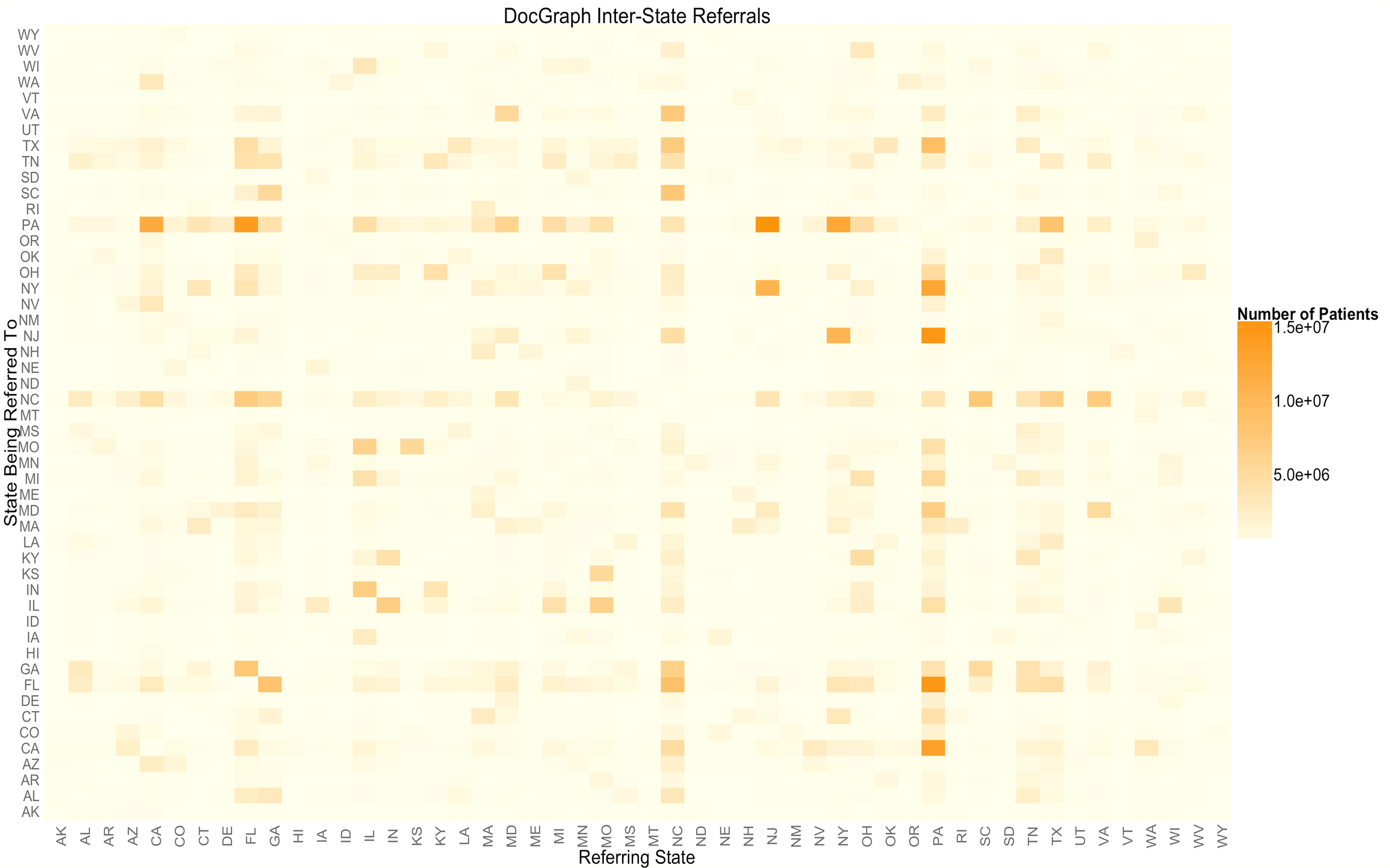
After analyzing the probability of inter-referrals I got curious where all these out-of-state referrals were going. As a first step towards understanding out-of-state referrals I assembled a heat map. This heat map provides some details on which states patients are being referred to. Each square in the heat map represents an entry in the state to state adjacency matrix contained in the DocGraph network.

The results above should have provide a good answer to the question of the impact of state on likelihood of out-of-state referrals. In addition we can get an idea of which states have the most inter-state referral traffic. Overall I think this analysis brings us one step closer to unlocking the potential of the DocGraph data to help us understand the U.S. health graph 1.

I hope you have enjoyed my analysis. I am always open to feedback and would love to collaborate on some research related to analyzing the DocGraph data set. If you are interested in collaborating on research related to DocGraph please email me ryan [at] weald.com or message me on twitter @rweald

#####Footnotes

1.

There are a couple of important limitations of the data to remember when interpreting this analysis. The DocGraph data set only includes data from 2011; we can assume that physician behavior is much the same today as it was in 2011, however without a sample from some other time period we can not be sure. Secondly, DocGraph only represents Medicare referrals which may not be representative of the entire healthcare system. Unfortunately a more comprehensive dataset including private referrals is not available to me at this time. Therefore, the DocGraph dataset is the best referral sample I could get as a private citizen.

2.

To create the final visualization I had to combine multiple data sets to enrich the doctor social graph with geographic coordinates. I began by taking a sample of 1 million connections from DocGraph and joining it with the National Provider Identifier (NPI) database. By joining these two data sets I was able to get the zip code of each physicians practice. The final step was converting the zip codes to latitude-longitude coordinates using a publicly available zip code database. Now that the data was in the correct format I began work on the visualization.

The visualization I choose was heavily inspired by the great work of Paul Butler at Facebook.

Using a similar method to the one documented in Nathan Yau’s tutorial I graphed the connections between physicians using great circles. In order to see the cluster density I layered the connections using Euclidean distance, with the longest paths being drawn first. All of the code used to generate this visualization is open source and can be found on Github

Below is the resulting visualization. Note the areas of high and low density as you move from the east coast over to the west coast. There are also some interesting connections from Hawaii and Puerto Rico to the Continental United States.

You can download the full sized graphic here. I recommend you right-click and “save link as” because the file is approximately 40MB.

This visualization is only the beginning. The added feature of geography opens the door to many interesting analyses. I would love to collaborate on some research related to analyzing the DocGraph data set. If you are interested in collaborating on research related to DocGraph please email me ryan [at] weald.com or message me on twitter @rweald

You can view the slides on Speaker Deck

Abstract:

I walk you through the basics of linear regression, and show you how you can perform simple linear regression using Ruby

The driving principle behind this post is “Banking your profits”. In software development that means making small focused commits on your master branch and using continuous integration[1] to get those small changes integrated with the rest of your production code. By banking these profits along the way you gaining value even if you never succeed with the larger effort.

So how can you possibly make small focused commits when you are working on an undertaking as monumental as a Rails 3 upgrade? The key to our success was small short lived Branches. The rules that governed these branches are as follows:

1) No branch may live longer than 24 hours

2) You can not make any unnecessary changes that could not be backported.

Following these rules you are able to shift your mindset. Rather than an all or nothing sprint we instead methodically identified technical debt that was hindering the upgrade but not directly a result of Rails API incompatibilities. It was really quite amazing how much of the upgrade pain was actually the result of tight coupling and SOLID[2] design principle violations rather than Rails 3 incompatibilities.

Whenever we encountered a piece of debt that was hindering our upgrade we would switch back to the master branch and fix the code. Following this method the all or nothing part of the upgrade only took 2 days! The best part was even if we had never succeeded on the final portion of the upgrade we would have drastically improved the quality of the code allowing the team to move faster.

If you follow the technique outlined here you will improve the quality of your codebase regardless of whether the upgrade is successful.

P.S.

Want to work with me tackling hard problems across the stack using TDD and pair programming? Sharethrough is hiring talented engineers

[1] https://en.wikipedia.org/wiki/Continuous_integration

[2] https://en.wikipedia.org/wiki/SOLID_(object-oriented_design)

1) Add mongoid to your gemfile

  gem "mongoid", "~> 2.0"
  gem "bson_ext", "~> 1.3"

2) Run the mongoid generator in your projects root directory

rails generate mongoid:config

This will generate a config/mongoid.yml file where you can configure your connection to mongodb.

3) Right now mongoid has overriden activerecord as the default orm so any attempts to generate migrations or ActiveRecord models will fail. Therefore we must configure our default generators so we can still use activerecord.

To do that simple add the following line to your config/application.rb file

  config.generators do |g|
    g.orm :active_record
  end

The reason for this is because Rails is an inherently I/O blocking. When you run your application in production using Passenger or Unicorn you essentially fork worker processes which are each responsible for servicing 1 requests at a time. To prevent memory bloating if a worker takes to long to respond or consumes too much memory it is killed. Well that presents a bit of a problem when you are talking about streaming file uploads that will require an active connection be left open while the file is uploaded. This large file upload request will block one of our worker processes which present an interesting problem. Since our process is blocked it is unable to service any additional request. This will lead to serious response time issues as our worker will be tied up handling these slow requests. To solve this we could spin up more worker processes, but this in turn takes more memory and more CPU and more resources in general.There must be a simpler solution!

It turns out there is in fact a simpler solution…Event Driven Programming and the Reactor Pattern. I know what you are thinking, He’s talking about NodeJS. Well yes and no, NodeJS is indeed a javascript event based asyncronous web server. However, I like ruby and I want to program my web service in ruby so where does that leave me; Eventmachine. EventMachine is a c++ based event-processing library with a rich ruby API that allows for event oriented programming using an event loop and callbacks. Programming a web service using EventMachine can be a little bit of a pain in the ass as your code quickly starts to look like spaghetti and that is where Goliath comes in.

Goliath is described as “Non-blocking, Ruby 1.9 Web Server.” It supports the full rack API and utilizes ruby 1.9.2’s fibers to make readable top down code. If you want to learn more you can check out some great articles by Ilya Grigorik. Essentially goliath gives us a great way to write code that follows a top down flow and it easy to read, but in reality it is running asynchronously using EventMachine. Now what the heck does that mean to me you ask. Well what that means is in under 30 lines of code I was able to write an asynchronous file upload server.

And here it is:

This was just my first plunge into the world of Non-blocking evented code so I am by no means an expert. If you see that I have made a terrible mistake or just want to give me some pointers feel free to do some. Just remember I am still young and while my college peers were out partying I was writing this code so try and make all criticism constructive

In my next post I will document the upload client that also takes advantaged of EventMachine and fibers to compute checksums and upload files to the web service.

To remidy this problem we decided to route the search request through our own application servers. Although at first glance this might appear to be a bad idea as it would increase latency, it turns out it actual decreased the average latency. The cause for this decrease in latency; caching. It turns out that most users enter the same search term almost every time they enter a citation. With this in mind we wrote some code in our application that caches the responses from mendeley API that way for any given search query we only have to make 1 request to the mendeley API. All subsequent requests for the search term will be returned from our application cache rather than a request to the API.

Caching was also a resonable solution for this particular problem because the mendeley search results change very infrequently.

You can see the code below that was used to cache the mendeley API response using whatever cache Rails is configured to use.

####The Code

def self.search_mendeley(query=nil)
  raise "no query specified" unless query

  papers = Rails.cache.fetch(query) do |query|
    response = Mendeley::API::Documents.search(query)
    papers = response["documents"][0..5]
  end

  return papers
end

The main difference between geo queries and your average run of the mill query is the need for and index. Normally when a simple unit test suite is run you don’t worry about building indexes as you wont be querying large amounts of data to speed is not an issue. Besides if you are reading this you are using Rspec which means you are not too concerned with your test speed.

However, if you want to test geo queries in MongoDB you will have to ensure that your index is built or the query can not be executed. This is because geospatial queries can only be run against a special 2D index and not against the underlying data.

Now the obvious solution would be to place some code in your spec_helper file that will create the indexes. I felt like this was a bit to heavy handed since I only wanted to test the geospatial queries in 1 describe block.

So to fix the problem I choose to add a call to Mongoid::Indexes create_indexes method within my before block.

describe ".guides_nearby" do
  before(:each) do
    @guide = Factory(:guide)
    Guide.create_indexes
    @result = Guide.guides_nearby("San Diego,United States")
  end
  it {@result.first.should == @guide}
end